
The Akaike Information Critera (AIC) is a widely used measure of a statistical model. It basically quantifies 1) the goodness of fit, and 2) the simplicity/parsimony, of the model into a single statistic.
When comparing two models, the one with the lower AIC is generally “better”. Now, let us apply this powerful tool in comparing various ARIMA models, often used to model time series.
The dataset we will use is the Dow Jones Industrial Average (DJIA), a stock market index that constitutes 30 of America’s biggest companies, such as Hewlett Packard and Boeing. First, let us perform a time plot of the DJIA data. This massive dataframe comprises almost 32000 records, going back to the index’s founding in 1896. There was an actual lag of 3 seconds between me calling the function and R spitting out the below graph!


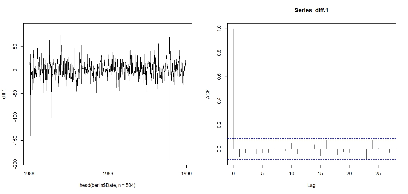
The first difference is thus, the difference between an entry and entry preceding it. The timeseries and AIC of the First Difference are shown below. They indicate a stationary time series.
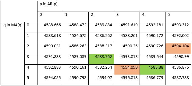
The AIC works as such: Some models, such as ARIMA(3,1,3), may offer better fit than ARIMA(2,1,3), but that fit is not worth the loss in parsimony imposed by the addition of additional AR and MA lags. Similarly, models such as ARIMA(1,1,1) may be more parsimonious, but they do not explain DJIA 1988-1989 well enough to justify such an austere model.
Note that the AIC has limitations and should be used heuristically. The above is merely an illustration of how the AIC is used. Nonetheless, it suggests that between 1988 and 1989, the DJIA followed the below ARIMA(2,1,3) model:

Next: Determining the above coefficients, and forecasting the DJIA.
Analysis conducted on R. Credits to the St Louis Fed for the DJIA data.
Abbas Keshvani

Hello there!
It’s again me.
As you redirected me last time on this post. I wanted to ask why did you exclude p=0 and q=0 parameters while you were searching for best ARMA oder (=lowest AIC).
I am asking all those questions because I am working on python and there is no equivalent of auto arima or things like that.
Thanks anyway for this blog
Hi! It’s because p=0, q=0 had an AIC of 4588.66, which is not the lowest, or even near.
If you find this blog useful, do tell your friends!
Hello Abbas!
i have two questions.
1. What is the command in R to get the table of AIC for model ARMA?
2. If the values AIC is negative, still choose the lowest value of AIC, ie, that -140 -210 is better?
Thank for your help.
Hi Daniel,
1. There is no fixed code, but I composed the following lines:
aic<-matrix(NA,6,6)
for(p in 0:5)
{
for(q in 0:5)
{
a.p.q<-arima(timeseries,order=c(p,0,q))
aic.p.q<-a.p.q$aic
aic[p+1,q+1]<-aic.p.q
}
}
aic
2. You can have a negative AIC. Pick the lower one.
If you like this blog, please tell your friends.
Hi Abbas!
I have 3 questions:
I come to you because usually you explain things simplier with simple words.
1)Can you explain me how to detect seasonality on a time series and how to implement it in the ARIMA method?
2)Also I would like to know if you have any knowlege on how to choose the right period (past datas used) to make the forecast?
3) Finally, I have been reading papers on Kalman filter for forecasting but I don’t really know why we use it and what it does?
Can you help me ? Thanks
🙂
In addition to my previous post I was asking a method of detection of seasonality which was not by analyzing visually the ACF plot (because I read your post : How to Use Autocorreation Function (ACF) to Determine Seasonality?)
My goal is to implement an automatic script on python.That’s why I am asking!
Thanks for answering my questions (lol,don’t forget the previous post)
🙂
Hi SARR,
1) I’m glad you read my seasonality post. I posted it because it is the simplest, most intuitive way to detect seasonality. For python, it depends on what method you are using. I personally favor using ACF, and I do so using R. You can make the process automatic by using a do-loop. See my response to Daniel Medina for an example of a do-loop.
2) Choose a period without too much “noise”. You want a period that is stable and predictable, since models cannot predict random error terms or “noise’. So choose a straight (increasing, decreasing, whatever) line, a regular pattern, etc…
3) Kalman filter is an algorithm that determines the best averaging factor (coefficients for each consequent state) in forecasting. If you’re interested, watch this blog, as I will post about it soon.
Tell your friends!
Abbas
Hi,
Nice write up. I am working on some statistical work at university and I have no idea about proper statistical analysis. But I found what I read on your blog very useful. Thanks for that.
I have a doubt about AIC though. I am working on ARIMA models for temperature and electricity consumption analysis and trying to determine the best fit model using AIC. All my models give negative AIC value. For example, I have -289, -273, -753, -801, -67, 1233, 276,-796. I know the lower the AIC, it is better. But in the case of negative values, do I take lowest value (in this case -801) or the lowest number among negative & positive values (67)??
Hoping for your reply.
Cheers
Hi Vivek, thanks for the kind words. Use the lowest: -801.
Hi,
Thank you for enlightening me about aic. I have a question and would be glad if you could help me. Do you have the code to produce such an aic model in MATLAB?
Sorry Namrata. I do not use Matlab. Once you get past the difficulty of using R, you’ll find it faster and more powerful than Matlab.
thank you
Hi Abbas,
Thanks for this wonderful piece of information. I have few queries regarding ARIMA:
1. Why do we need to remove the trend and make it stationary before applying ARMA? Won’t it remove the necessary trend and affect my forecast?
2. Apart from AIC and BIC values what other techniques we use to check fitness of the model like residuals check?
3. What are the limitation (disadvantages) of ARIMA?
Sorry for trouble but I couldn’t get these answers on Google.
Thanks a lot,
Deepesh Singh
Thanks for the kind feedback Deepesh.
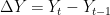
A simple ARMA(1,1) is Y_t = a*Y_(t-1) + b*E_(t-1).
Now Y_t is simply a constant [times] Y_(t-1) [plus] a random error. The error is not biased to always be positive or negative, so every Y_t can be bigger or smaller than Y_(t-1). The series is not “going anywhere”, and is thus stationary.
So any ARMA must be stationary. If a series is not stationary, it cannot be ARMA.
Hi Abbas,
How can I modify the below code to populate the BIC matrix instead of the AIC matrix?
aic<-matrix(NA,6,6)
for(p in 0:5)
{
for(q in 0:5)
{
a.p.q<-arima(timeseries,order=c(p,0,q))
aic.p.q<-a.p.q$aic
aic[p+1,q+1]<-aic.p.q
}
}
aic
thank you so much for useful code.now i don’t have to go through rigourous data exploration everytime while doing time series
If the lowest AIC model does not meet the requirements of model diagnostics then is it wise to select model only based on AIC?
Hi Abbas,
Could you please let me know the command in R where we can use d value obtained from GPH method to be fitted in ARFIMA model to obtain minimum AIC values for forecast?
fracdiff function in R gives d value using AML method which is different from d obtained from GPH method.
Hi Sir,
I am working to automate Time – Series prediction using ARIMA by following this link https://github.com/susanli2016/Machine-Learning-with-Python/blob/master/Time%20Series%20Forecastings.ipynb
I have a concern regarding AIC value. In the link, they are considering a range of (0, 2) for calculating all possible of (p, d, q) and hence corresponding AIC value. And for AIC value = 297 they are choosing (p, d, q) = SARIMAX(1, 1, 1)x(1, 1, 0, 12) with a MSE of 151.
Now when I increase this range to (0, 3) from (0, 2) then lowest AIC value become 116 and hence I am taking the value of the corresponding (p, d, q) but my MSE is 34511.37 which is way more than the previous MSE.
I am unable to understand why this MSE value is so high if I am taking lower AIC value.
Any help would be highly appreciated.
Thanks,
Girijesh Singh
Hey, I wonder for this case: why not use the AMIMA(1,1,1) model?
It seems that ARIMA(2,1,3) is only ~0.02% better in AIC , but has a way less interpretable result. Further the ACF of our TS is not significant for any lags except for the first one (and maybe conincidentally for the 23rd one), so I wonder if our model selection is justified…
I have no idea what the AIC actually measures, so I don’t know how to interpret it, but can you give me an intuition for the ACF result?
Many thanks!