In my previous post, I wrote about using the autocorrelation function (ACF) to determine if a timeseries is stationary. Now, let us use the ACF to determine seasonality. This is a relatively straightforward procedure.
Firstly, seasonality in a timeseries refers to predictable and recurring trends and patterns over a period of time, normally a year. An example of a seasonal timeseries is retail data, which sees spikes in sales during holiday seasons like Christmas. Another seasonal timeseries is box office data, which sees a spike in sales of movie tickets over the summer season. Yet another example is sales of Hallmark cards, which spike in February for Valentine’s Day.
The below graphs show sales of clothing in the UK, and how these sales follow seasonal trends, spiking in the holiday season:

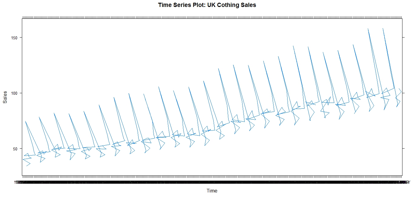
Note the spikes in sales, which obediently occur every December, in time for Christmas. This is evident in the trail of December plot points (Graph 1), which hover significantly above the sales data for other months, and also in the actual spikes of the line graph (Graph 2).
The above is a simple example of a seasonal timeseries. However, timeseries are not always simply seasonal. For example, a SARMA process comprises of seasonal, autoregressive, and moving average components, hence the acronym. This will not look as obviously seasonal, as the AR and MA processes may overlap with the seasonal process. Thus, a simple timeseries plot, as shown above, will not allow us to appreciate and identify the seasonal element in the series.
Thus, it may be advisable to use an autocorrelation function to determine seasonality. In the case of seasonality, we will observe an ACF as below:
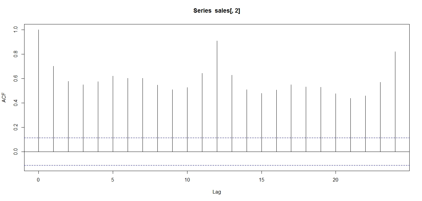
Note that the ACF shows an oscillation, indicative of a seasonal series. Note the peaks occur at lags of 12 months, because April 2011 correlates with April 2012, and 24 months, because April 2011 correlates with April 2013, and so on.
The above analyses were conducted on R. Credits to data.gov.uk and the Office of National Statistics, UK for the data.
Abbas Keshvani

Excellent commentary on seasonality using ACF.
Thank you!
Dear Abbas,
Would I please be able to use your ACF function plots for seasonality and stationarity for my dissertation? Just as a point of reference.
Thanks,
Jay
Sure
Excellent explanations! But I wonder how you can get the information of the peiriod, here 12 month, without read it on the ACF graph? Can you help me? I have a time seires with an unknow period….
Hi Hugo, look at your ACF. The period is the first spike that stands out.
I know my clothing data has a period of 12, since the ACF spikes at the 12th lag.
Thank you…good explanation!!!
Thanks!
Dear Abbas,
Thanks for explaining usage of ACF to find seasonality. I have two questions
1) If there exists no seasonality in data, how can it be identified? Since ACF will still give spikes may be with smaller range. What should be cutoff value or threshold value for considering the spike as significant from others. Also does it guarantee presence/ absence of seasonality.?
2) In real world, datasets would have noise and hence while predicting the period using ACF might take that as well into consideration, because it might affect in computing period.
Thanks and Regards,
-Vikrant
Thanks Vikrant.
1. An ACF spike at lags of 4 means that there is a strong correlation between every 4th point. It indicates seasonality. But if the correlation is strong for all points, then it means that the series is just non-stationary or random.
2. ACF tells you the correlation between every single point and its k-th lag. Noise cannot affect the entire data series to show a false correlation.
Thanks for this explanation. I have two questions.
1. Can it be said that the ACF plotted above depicts a non-stationary time series?
2. Is every seasonal time series non-stationary?
1. No, it is stationary. Please see here for details: https://coolstatsblog.com/2013/08/07/how-to-use-the-autocorreation-function-acf/
2. No, stationary series can also have a seasonal component. I.e. the series is stable over time and there is a spike every December.
Thanks for visiting!
what a clear explanation, thank you!
This is extremely helpful! I have a question though. How can you tell from your ACF graph whether the time series has additive seasonality or multiplicative?
I am personally working on some forecasting work and I’ve got a time series that peaks at every 12 months but the size of the oscillations decreases. The original time plot suggests there’s multiplicative seasonality so is this what the ACF plot is confirming?
Thanks in advance!
Thank you Abbas, for your interesting and useful notes. From the conceptual point of view, it seems that seasonality is a multiplicative component in the process because the seasonality effect depends on the previous amount of signal. I mean additive component are uncorrelated with the original signal yet seasonality is correlated with original signal.
can I ask if the spike seen in 11 and 24, 34 ?? is this seasonal?
Thanks Abbas for a clear explanation. I want to automate the process so that I can get to know which all products have seasonality out the data set of 10000 products I have. I can’t see the graph of each and every product to decide seasonality due to the lack of time and sheer volume of the products. Please guide me through this
Hi,
Could you help me with how to interpret the following values: –
Time lag k ACF(k) T-STAT P-value
1 0.189758 0.8051 0.215642
2 -0.058458 -0.248 0.403465
3 -0.185316 -0.7862 0.220981
4 -0.116981 -0.4963 0.312842
5 -0.099142 -0.4206 0.339505