The Autocorrelation function is one of the widest used tools in timeseries analysis. It is used to determine stationarity and seasonality.

Stationarity:

This refers to whether the series is “going anywhere” over time. Stationary series have a constant value over time.

Below is what a non-stationary series looks like. Note the changing mean.

And below is what a stationary series looks like. This is the first difference of the above series, FYI. Note the constant mean (long term).

The above time series provide strong indications of (non) stationary, but the ACF helps us ascertain this indication.

If a series is non-stationary (moving), its ACF may look a little like this:

The above ACF is “decaying”, or decreasing, very slowly, and remains well above the significance range (dotted blue lines). This is indicative of a non-stationary series.

On the other hand, observe the ACF of a stationary (not going anywhere) series:

Note that the ACF shows exponential decay. This is indicative of a stationary series.

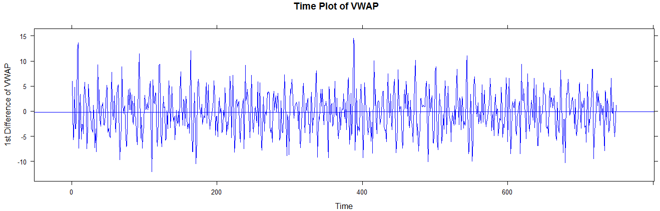
Consider the case of a simple stationary series, like the process shown below:

We do not expect the ACF to be above the significance range for lags 1, 2, … This is intuitively satisfactory, because the above  process is purely random, and therefore whether you are looking at a lag of 1 or a lag of 20, the correlation should be theoretically zero, or at least insignificant.

Next: ACF for Seasonality

Abbas Keshvani