Random Variables from a non-Parametric distribution know their limits

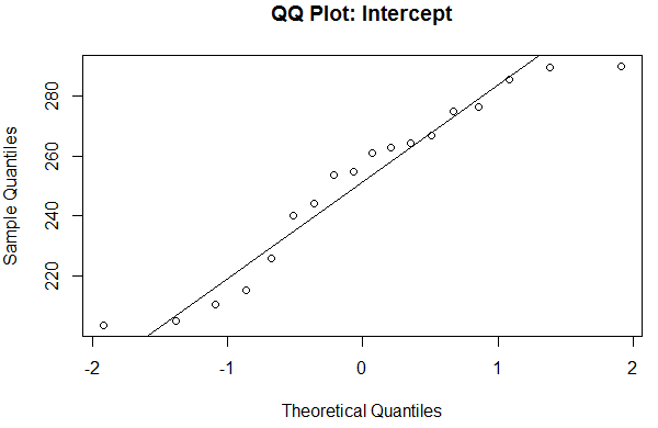
You produce a non-parametric distribution. Then you obtain, say, 10 random variables (RV) from this non-parametric distribution- much the same way as you would obtain random variables from a (parametric) normal distribution with stated mean and variance. But unlike the parametric distribution, where our RVs would occur around the mean (our parameter), RVs from a non-parametric distribution occur within the range bound by the lowest and highest mass point. This was not necessarily an intuitive concept to me, when I first stumbled across it. Which is why this mathematical proof of this range made me feel so much more comfortable:

If our estimate of the RV is a simple weighted-mean of the mass points:

$\hat{\beta} = z_{1}w_{1} + ... + z_{k}w_{k}$

Furthermore, since $z_1 \leq \hat{\beta} \leq z_k$ for RV $\beta$ :

$\left[w_{1}+...+w_{k} \right]z_{1}\leq \hat{\beta}\leq \left[w_{1}+...+w_{k} \right]z_{k}$

Since $\sum w_i=1$ , we can express the inequality as:

$z_1 \leq \hat{\beta} \leq z_k$

On the other hand, If we know further information, like individual weights:

$\hat{\beta}=z_1w_1+...+z_kw_k$

Furthermore, since for intercept $\beta$ :

$\left(w_{1}+w_{k}\right)z_1\leq \hat{\beta}\leq \left(w_{1}+w_{k}\right)z_k$

Since $\sum w_i=1$ , we can express the inequality as:

$z_1\leq \hat{\beta}\leq z_k$

Thus, it is proven that any estimates of an RV drawn from a non-parametric distribution will be bound by the highest and lowest mass point.

Abbas Keshvani

Limits of Akaike Information Criteria (AIC)

We often use AIC to discern the best model among candidates.

Now suppose we have two (non-parametric) models, which use mass points and weights to model a random variable:

model A uses 4 mass points to model a random variable (i.e. the height of men in Singapore)
model B uses 5 mass points to mode the same random variable

We consider model A to be nested in model B. This is because model A is basically a version of model B, where one mass point is “de-activated”.

Thus, we must not use small differences in AIC or BIC alone to judge between these models. If the model with a constraint on one or more parameters (model A) is regarded as nested on within the model without the constraint (model B) , a chi-square difference test, or Likelihood Ratio (LR) test, is performed to test the reasonableness of the constraint, using a central chi-square with degrees of freedom equal to the number of parameters constraints.

However, under the null hypothesis, the parameter of interest takes its value on the boundary of the parameter space (next post). For this reason, the asymptotic distribution of the chi-square difference, or Likelihood Ratio (LR) statistic, is not that of a central chi-square distributed random variable with one degree of freedom. This boundary problem affects goodness of fit measures like AIC and BIC4. As a result, the AIC and BIC should be used heuristically, in conjunction with graphs and other criteria to evaluate estimates from the chosen model.

Abbas Keshvani

Parametric vs non-Parametric Linear Models (LM)


Histogram: LM estimates of Intercepts	Histogram: LM estimates of Gradient

QQ Plot: LM estimates of Intercepts	QQ Plot: LM estimates of Gradient

Figure 1: Gradient appears to follow a normal distribution more than intercept .

When do we use a parametric model, and when do we use a non-parametric one? In the above example, “Intercept” is one random variable, and “Gradient” is another. I will show you why “Intercept” is better modeled by a non-parametric model, and “Gradient” is better modeled by a parametric one.

In Figure 1, histograms and QQ plots of “Intercept” and “Gradient” show that the latter appears to follow a normal distribution whereas the former does not. As such, a parametric (normal) distribution would not be appropriate for modelling “Intercept”. This leads us to believe that a non-parametric distribution is a better method for estimating “Intercept”.

However, a parametric (normal) distribution might be appropriate for modelling “Gradient”, which appears to follow a normal distribution, according to both its histogram and QQ plot.

Abbas Keshvani