Suppose you have decided on a suitable model for a timeseries. In this case, we have selected an ARIMA(2,1,3) model, using the Akaike Information Criteria (AIC) as our sole criterion for choosing between various models here, where we model the DJIA.
Note: There are many criteria for choosing a model, and the AIC is only one of them. Thus, the AIC should be used heuristically, in conjunction with t-tests and the Coefficient of Determination, among other statistics. Nonetheless, let us assume that we ran all these tests, and were still satisfied with ARIMA(2,1,3).
An ARIMA(2,1,3) looks like this:
This is not very informative for forecasting future reaizations of a timeseries, because we need to know the values of the coefficients ,
, etcetera. So we use R’s arima() function, which spits out the following output:

Thus, we revise our model to:
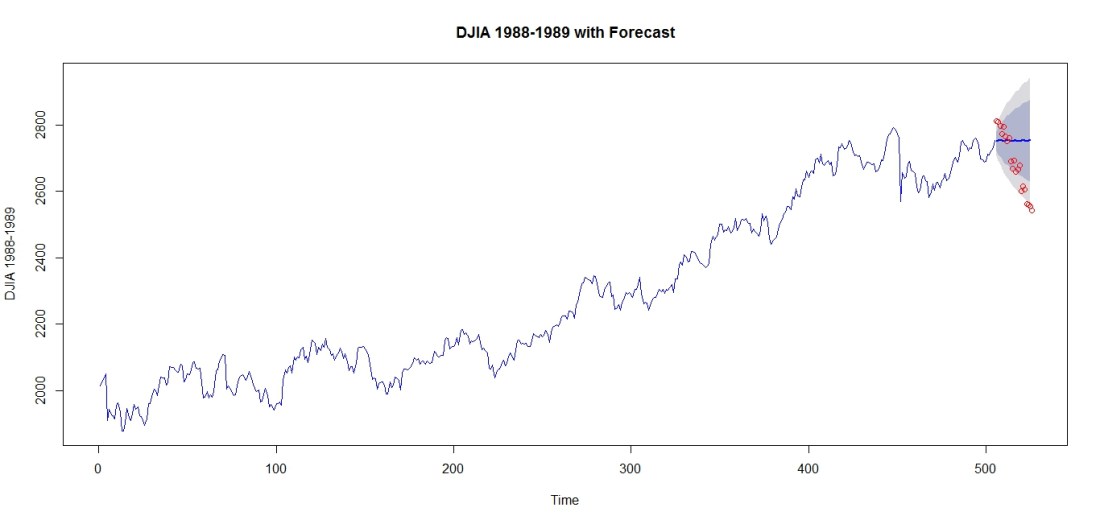
Then, we can forecast the next, say 20, realizations of the DJIA, to produce a forecast plot. We are forecasting values for January 1st 1990 to January 26th 1990, dates for which we have the real values. So, we can overlay these values on our forecast plot:

Note that the forecast is more accurate for predicting the DJIA a few days ahead than later dates. This could be due to:
- the model we use
- fundamental market movements that could not be forecasted
Which is why data in a vacuum is always pleasant to work with. Next: Data in a vacuum. I will look at data from the biggest vacuum of all – space.